
- A NEW WAY OF RENDERING FRAMES
- A BRIEF DISCUSSION OF SHADERS & SPLITTING THE WORLD AND VIEWPROJ MATRICES
- DESCRIPTOR HEAPS
- OBJECT MANAGEMENT AND WHERE DO WE GET THE DATA FROM?
A NEW WAY OF RENDERING FRAMES
Well things certainly have moved on quite a bit. Since the last chapter I’ve added some more very useful things from the textbook I’m referring to, which we’ll be relying heavily upon during this chapter (see previous chapters for textbook details – and buy the book). I’ve also rebuilt a fair sized portion of the rendering library. Needless to say I’ve also had to fix a lot of bugs, as always happens when adding new parts to your project, or overhauling existing parts of it. The rather ugly video below shows the project in its latest state, and what this article will be about.
I could not get the video quality any better without causing frame rates to drop terribly. Perhaps it really is time I invested in some new hardware. Anyways, it shows well enough what’s happening and that’s all we’re really interested in. What you see in the video below is the new way of handling rendering using multiple frame resources in a circular array (which improves performance) and also the project’s object management functions working correctly. The object management will trigger when we attempt to add more objects to the scene than we have allowed for, and will choose the object furthest from the camera to be removed from rendering in favour of a new one that is nearer to the camera.
This happens whenever you press the F2 key during running. In this example it allows the addition of up to four new objects into a scene rendering 12 cubes rotating around the centre. As each new cube is added in the middle, one is removed from the outer circle. This keeps the amount of objects we render in a scene fixed to a value we’ve chosen. Given that this project is ultimately intended to do only what’s needed, and also run reasonably well on low end machines, this is important before considering future developments. Notice that each time a cube is removed from the outer circle it’s always the one furthest from the camera. That’s why I added the rotation to demonstrate this.
So I probably do have quite a bit more to learn when it comes to mastering video capturing. It’s not really my main aim, but I will try and improve it over time. For now though, functional is good enough.
Now we’ll discuss the first new thing in the project which is the multiple frame concept. In previous chapters we used to render stuff by loading a load of commands into the command queue and then flushing it. Whilst it was being flushed we waited. When the GPU stated it was ready, we continued onwards and processed the next frame. This can causes rather a lot of waiting though. We deal with two processors, the CPU and the GPU. The CPU is doing most of the work you can see in the code, such as creating variables and calling functions, filling buffers with data etc.. The GPU is doing all the actual drawing with the data we load into it. They’re not synchronised in any standard or default way. They just continue on doing their work, and we add code that causes our program to wait until the GPU is ready to receive more commands.
Conversely if the GPU is already finished when we call the function that flushes the command queue it means the GPU has been idling waiting for the CPU. In the latest chapter of the textbook the author has decided to do something a bit better than that. In previous chapters we had the stuff we needed to just render one frame at a time. We’d have a vertex buffer, an index buffer, a descriptor heap with views/descriptors in it and so on. We just referred to them whenever we needed them, and they were all in their respective places dotted about the project (wherever made the most sense to store them at the time).
In the new way of doing things, everything we need (or most of them) for a frame to be rendered, is kept inside its own structure. This means we can have multiple frames each with their own resources. The idea of keeping a frame self-contained like that, is that you can render multiple frames independently from each other. Each frame has all the stuff it needs to make one pass on the graphics card.
You may ask why would you want to do that? The reason is, it allows the CPU to load the commands for multiple frames at a time, instead of just loading one and then waiting for the GPU to catch up before continuing. So several complete frames worth of commands are loaded into the queue at a time. The GPU then chews through them all signalling when it has completed each one. Note that the GPU signals when it has complete each frame. This allows us to keep track of exactly which frames have been processed by the GPU. This is needed when we use a function to see whether or not we need to wait for the GPU before continuing loading more data.
Before we get too carried away with that, lets have a look at what a Frame Resource structure actually looks like, and note that we have 3 of them in the project.
// Stores the resources needed for the CPU to build the command lists
// for a frame.
struct FrameResource
{
public:

    FrameResource(ID3D12Device* device, UINT passCount, UINT objectCount);
    FrameResource(const FrameResource& rhs) = delete;
    FrameResource& operator=(const FrameResource& rhs) = delete;
    ~FrameResource();

    // We cannot reset the allocator until the GPU is done processing the commands.
    // So each frame needs their own allocator.
    Microsoft::WRL::ComPtr<ID3D12CommandAllocator> CmdListAlloc;

    // We cannot update a cbuffer until the GPU is done processing the commands
    // that reference it.  So each frame needs their own cbuffers.
    std::unique_ptr<UploadBuffer<PassConstants>> PassCB = nullptr;
    std::unique_ptr<UploadBuffer<ObjectConstants>> ObjectCB = nullptr;

    // Fence value to mark commands up to this fence point.  This lets us
    // check if these frame resources are still in use by the GPU.
    UINT64 Fence = 0;
};
So it has a constructor function, then some stuff that prevents copy constructors and its destructor. Then you’ll notice it has its own command allocator, and two upload buffers, then finally a fence value. Each frame absolutely can have its own command allocator, despite the fact the project uses only one command queue and one command list. So it seems a queue can accommodate multiple allocators. The only requirement will surely be that they are sent to the queue contiguously. So we use our command list to record to each frame’s allocator, and each frame’s allocator is then added to the queue.
So maybe the picture is becoming a bit clearer here. We’re going to record to each frame’s allocator at a time then move on to the next, and when we’ve recorded to all three we return to the first and see if the GPU has caught up yet (i.e. finished processing all the commands for that frame). So each time the main Draw() function is executed in the project it will be referencing a different frame each time. Care obviously needs to be taken here to make sure command lists are closed when recording is finished, and allocators don’t get over-written when they haven’t finished being read yet (this will cause a crash). The crucial concept here is, as stated above, that the Draw() function is referencing a different frame each time it runs. I struggled with this at first, it’s almost as bad as function recursion to try and picture in your mind.
To make use of three frames and pass over them continuously before returning to the first we use a circular array of size 3, with obviously indexes of 0, 1, and 2.
// Frame resource data members
std::vector<std::unique_ptr<FrameResource>> mFrameResources;

// ....some time later
const int gNumFrameResources = 3;

// .....more time later

void D3DRenderer::BuildFrameResources()
{
    for (int i = 0; i < gNumFrameResources; ++i)
    {
	mFrameResources.push_back(std::make_unique<FrameResource>(md3dDevice.Get(),
			1, 1));
    }
}
That builds our array of 3 Frame Resources (I may refer to Frame Resources in lower case from now on). Now how does each frame resource keep track of its data member fence value? Surely it needs to be incremented each time a frame is processed? And it is, in the Draw() function. Below is a small snippet of where that happens. Bear in mind mCurrentFence is initialised to zero in the main render class:
// inside D3DRender class

UINT mCurrentFence = 0;
// function Draw() ....after all drawing commands are complete
// Advance the fence value to mark commands up to this fence point.
mCurrFrameResource->Fence = ++mCurrentFence;
// Add an instruction to the command queue to set a new fence point.
// Because we are on the GPU timeline, the new fence point won't be
// set until the GPU finishes processing all the commands prior to this Signal().
mCommandQueue->Signal(mFence.Get(), mCurrentFence);So each time the Draw() function is called the D3DRender class data member mCurrentFence is incremented and the current frame resource (either 0, 1, or 2 – whichever frame is current) has its fence value set to mCurrentFence.
So for example the very first time this is run and the Draw() function is called for the first time, it will load all the commands into the allocator via the list and then instruct those commands to be executed, and then after that it increments the D3DRender class data member mCurrentFence from 0 to 1, and also set the current frame resource’s fence to 1.
The last thing to discuss here before we move to a picture demonstration of this, is exactly which of the frames 0, 1, or 2 this circular array beings with. This is determined in the first call to the Update() function in the render class. Note that Update() is called before Draw():
// ....earlier in D3DRender class
int mCurrFrameResourceIndex = 0;

void D3DRenderer::Update(const GameTimer& gt)
{
    // Cycle through the circular frame resource array.
    mCurrFrameResourceIndex = (mCurrFrameResourceIndex + 1) % gNumFrameResources;
    mCurrFrameResource = mFrameResources[mCurrFrameResourceIndex].get();

    ....function continues
Obviously we can see that (1 % 3) resolves to 1. So the first frame we will actually process is index 1 in the mFrameResources array, not zero. So it looks a little bit like this in conception:
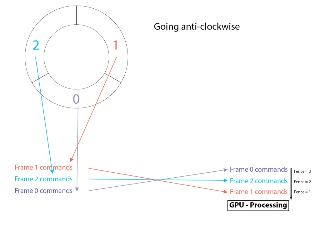
So you can see that each frame’s commands are loaded into the GPU, one on top of the other, and as the Draw() function is called for each frame, that frame’s fence value gets updated. The last thing to consider is the part of the Update() function we have not shown yet. This is where the CPU either waits for the GPU or just continues onwards.
void D3DRenderer::Update(const GameTimer& gt)
{
    static int frames = 0; // used to show us how many times in the first 1000 frames
                           // we've had to wait for the GPU. We want this number to be
                           // fairy high.

    // Cycle through the circular frame resource array.
    mCurrFrameResourceIndex = (mCurrFrameResourceIndex + 1) % gNumFrameResources;
    mCurrFrameResource = mFrameResources[mCurrFrameResourceIndex].get();

    // Has the GPU finished processing the commands of the current frame resource?
    // If not, wait until the GPU has completed commands up to this fence point.
    if ( (mCurrFrameResource->Fence != 0) && (mFence->GetCompletedValue() < mCurrFrameResource->Fence) )
    {
        HANDLE eventHandle = CreateEventEx(nullptr, false, false, EVENT_ALL_ACCESS);
        ThrowIfFailed(mFence->SetEventOnCompletion((mCurrFrameResource->Fence),
                                                    eventHandle));
        WaitForSingleObject(eventHandle, INFINITE);
        CloseHandle(eventHandle);
        if (frames < 1000) { mGPUWaitOccurences++; }
    }

    frames++;

    UpdateObjectCBs();
    UpdatePassCBs(gt);

    return;
}
So we can see for the first 3 passes the GPU is not waited for, as each frame resource’s fence starts at zero. After the third pass we are back to index 1 in the array (more specifically a vector) where we began. The if statement will be entered now if the GPU hasn’t caught up. That’s what the GetCompletedValue() function does. If the fence currently completed on the GPU timeline is equal to or greater than the fence number stored in that frame resource, we know the GPU has moved past this frame already. If it hasn’t, we wait until it has. You can see that for the next three passes each frame resource’s fence is incremented to 4, 5 and 6 respectively.
That’s as much as we’re going to discuss about this concept in this chapter. A more detailed explanation is available in the recommended textbook.
A BRIEF DISCUSSION OF SHADERS & SPLITTING THE WORLD AND VIEWPROJ MATRICES
In previous projects we made the worldViewProj matrix on the CPU side and loaded it into the GPU through the constant buffer, where we then used it in the shader program. This time (as you may already have deduced) we split the worldViewProj matrix into two parts. The world matrix and the viewProj matrix. The world matrix goes into ObjectCB buffer you can see declared in the Frame Resource header file some ways above. The viewProj matrix goes in the PassCB buffer you can see declared in the line above it.
Each frame resource gets a copy of an object’s world matrix. This is what dictates the size of the UploadBuffer named ObjectCB. Here’s a sample of the Frame Resource constructor definition in the .cpp file (note the function argument objectCount isn’t used):
FrameResource::FrameResource(ID3D12Device* device, UINT passCount, UINT objectCount)
{
    ThrowIfFailed(device->CreateCommandAllocator(
        D3D12_COMMAND_LIST_TYPE_DIRECT,
        IID_PPV_ARGS(CmdListAlloc.GetAddressOf())));

    PassCB = std::make_unique<UploadBuffer<PassConstants>>(device, passCount, true);
    ObjectCB = std::make_unique<UploadBuffer<ObjectConstants>>(device, MAXOBJECTS, true);
};
In the root signature function we make it known we will be sending data to two registers for the shader program. One will be used for the ObjectCB and one for the PassCB. ObjectConstants and PassConstants are shown below:
struct ObjectConstants
{
    XMFLOAT4X4 world = MathHelper::Identity4x4();
};


struct PassConstants
{
    XMFLOAT4 light = XMFLOAT4(0.0f, 0.0f, 0.0f, 0.0f);
    XMFLOAT4X4 viewProj = MathHelper::Identity4x4();
};
So these values ultimately find their way into the shader program like this:
cbuffer cbPerObject : register(b0)
{
    float4x4 gWorld;
};

cbuffer cbPass : register(b1)
{
    float3 light;
    float4x4 gViewProj;
};
And then we combine them in the shader to produce the worldViewProj matrix we need to properly render the vertices.
DESCRIPTOR HEAPS
You may have been wondering what happens with the descriptors and descriptor heaps, given that we now have three frame resources each containing their own copy of object (world matrix) and camera (viewProj matrix) data. The descriptors/views are all simply fed into one large descriptor heap. I think I mentioned something about this above (I may not have), nevertheless we’ll cover it here also.
All object world matrices from each frame are bound to the descriptor heap in one go. The camera matrices (there only 3 of them – one for each frame) are simply added at the end. So Frame 0’s matrices occupy the first third of the descriptor heap’s data, and its camera matrix is just added to the first position at the end of all the object matrices. You may have to zoom in to see this more clearly in the picture below. Note (as already stated) that for the constant buffer views there is just one large descriptor heap laid out as shown below.
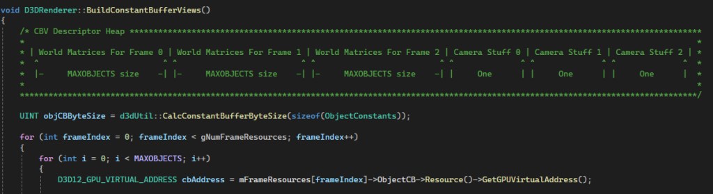
The heap is made in the D3DRenderer::CreateCbvDescriptorHeaps() function and the object and camera data is bound to it by the views created in the D3DRenderer::BuildConstantBufferViews() function. You can see those in the source code which is available for download at the end of this chapter.
OBJECT MANAGEMENT AND WHERE DO WE GET THE DATA FROM?
The data for the actual vertices is made in a very similar way to the last version of the project, if I’m recalling it correctly. There is a hierarchy in place here. The vertex data for each object is made in a function that loads all the vertices and indices into one large vertex buffer and index buffer respectively. We always refer back to this when we need the data to do the actual drawing.
Below this is the render items array. This is where we add objects we are intending to draw. But we may be adding several of the same type. We keep track of which type of object we’re rendering using the following structure (which I’ve altered slightly from the original one made by the textbook author):
// Lightweight structure stores parameters to draw a shape.  This will
// vary from app-to-app.
struct RenderItem
{
    RenderItem() = default;

    // World matrix of the shape that describes the object's local space
    // relative to the world space, which defines the position, orientation,
    // and scale of the object in the world.
    XMFLOAT4X4 World = MathHelper::Identity4x4();

    XMVECTOR Pos;

    // Dirty flag indicating the object data has changed and we need to update the
    // constant buffer.
    // Because we have an object cbuffer for each FrameResource, we have to apply the
    // update to each FrameResource.  Thus, when we modify object data we should set
    // NumFramesDirty = gNumFrameResources so that each frame resource gets the update.
    int NumFramesDirty = gNumFrameResources;

    // Index into GPU constant buffer corresponding to the ObjectCB for this render item.
    UINT ObjCBIndex = -1;

    MeshGeometry* Geo = nullptr;

    // Primitive topology.
    D3D12_PRIMITIVE_TOPOLOGY PrimitiveType = D3D_PRIMITIVE_TOPOLOGY_TRIANGLELIST;

    // DrawIndexedInstanced parameters.
    UINT IndexCount = 0;
    UINT StartIndexLocation = 0;
    int BaseVertexLocation = 0;
};
So it stores its world matrix and also its position in the scene, along with some other data needed for drawing. Note the last three data members at the bottom. These will be set to the relevant parts of the index and vertex buffers that hold the data for this render item. They’re connected to this data through another structure named MeshGeometry, which will not be shown here. You can find it in the book, or the source code. We have two unordered maps for the MeshGeometry structs in the main class:
std::unordered_map<std::string, std::unique_ptr<MeshGeometry>> mGridGeometry;
std::unordered_map<std::string, std::unique_ptr<MeshGeometry>> mBasicShapeGeometries;
One stores data for the grid, and the other for all the shapes. I probably could have combined both these categories into just one unordered map. At the moment we’re only using cubes (two cubes each of a different colour) in the same buffer. We’ll add other shapes in later versions however. Below is a snippet from the MeshGeometry struct which shows where the data gets mapped to whichever Submesh we require (whichever of the two different colour cubes we want).
// A MeshGeometry may store multiple geometries in one vertex/index buffer.
// Use this container to define the Submesh geometries so we can draw
// the Submeshes individually.
std::unordered_map<std::string, SubmeshGeometry> DrawArgs;
And a snippet of where we make one of these SubMeshGeometry structs in the function that builds all the vertex and index data:
SubmeshGeometry coralBoxSubmesh;
coralBoxSubmesh.IndexCount = (UINT)boxIndices.size();
coralBoxSubmesh.StartIndexLocation = coralBoxIndexOffset;
coralBoxSubmesh.BaseVertexLocation = coralBoxVertexOffset;
So we have one place where all the data is built and stored (a MeshGeometry), and the submeshes are defined for each shape’s vertices in the vertex buffer and its corresponding indices. This one struct holds several shape types in one buffer. The various submeshes are stored in unordered map called DrawArgs.
From there we have another struct that holds each individual shape we want to render (we may have several of the same type), and that shape takes an index in the array of items we are going to render (array of RenderItems named mAllRitems). That individual shape’s RenderItem struct then has the data members:
// DrawIndexedInstanced parameters.
UINT IndexCount = 0;
UINT StartIndexLocation = 0;
int BaseVertexLocation = 0;
filled out with data corresponding to the shape’s position in the MeshGeometry vertex and index buffer, depending upon which type of shape it is. In this project we use two. Both are cubes, one is coloured Coral and the other Orchid. Despite the fact they are both cubes, they still have different vertices due to the colour being different, so each needs its own unique place in the vertex buffer. They both use the same indices though. Here’s a snippet of a coral box being added to the array of RenderItems:
int D3DRenderer::AddRenderItems(geometryType& gType, basicShapesSubMesh& bSubMesh,
                                const float* translation, int index)

Name = "basicShapesGeo";

case CORAL_BOX:
{
    auto boxRitem = std::make_unique<RenderItem>();

    XMFLOAT3 position = XMFLOAT3(translation);
    boxRitem.get()->Pos = XMLoadFloat3(&position);

    boxRitem->Geo = mBasicShapeGeometries[Name].get();
    boxRitem->ObjCBIndex = index;
    XMStoreFloat4x4(&boxRitem->World, XMMatrixTranslation(translation[0],
                                                          translation[1],
                                                          translation[2]));

    boxRitem->PrimitiveType = D3D_PRIMITIVE_TOPOLOGY_TRIANGLELIST;
    boxRitem->IndexCount = boxRitem->Geo->DrawArgs["coralBox"].IndexCount;
    boxRitem->StartIndexLocation = boxRitem->Geo->DrawArgs["coralBox"]
                                                 .StartIndexLocation;
    boxRitem->BaseVertexLocation = boxRitem->Geo->DrawArgs["coralBox"]
                                                 .BaseVertexLocation;

....sometime later
    mAllRitems.push_back(std::move(boxRitem));
    boxRitem.release()
}
For the best view of how this all works you can study the source code, but that’s a reasonable overview of what’s happening.
The last thing to discuss is how we deal with adding an object to the render items array when the array is already at the max size we’ve allowed for. We simply search though all the items in the render items array and find the one with the largest distance to the camera and then remove it, and add the new item in its place.
Note there is actually a slight weakness in the function at this time. It doesn’t check to see if the new item being added is even further from the camera than any item already in the render items array. I’ll attempt to fix this for the next project revision. Note also its the same function as above, just a different part of it:
int D3DRenderer::AddRenderItems(geometryType& gType, basicShapesSubMesh& bSubMesh,
                                const float* translation, int index)
{
    float maxObjectDistFromCamera = 0.0f;
    float d;
    int maxDistIndex = 1000;

    if (mAllRitems.size() == MAXOBJECTS)
    {
	for (int i = 0; i < mAllRitems.size(); i++)
        {
            d = ObjectDistanceFromCamera(mAllRitems[i].get()->ObjCBIndex);
	    if (d > maxObjectDistFromCamera)
	    {
	        maxObjectDistFromCamera = d;
	        maxDistIndex = i;
	    }
        }

    index = maxDistIndex;
    RenderItem* pointer = mAllRitems[index].release();
    if(pointer != nullptr)(delete pointer);

....function continues
And that concludes everything that we’re going to discuss for this chapter. There is more to it however, but it would take far too long to discuss all changes to it here. For that, you need to study the source code. A link will be provided below. If you have any questions you can email me at links I’ve provided to my e-mail address in earlier chapters. Thank you for reading 🙂
