LINK ERROR

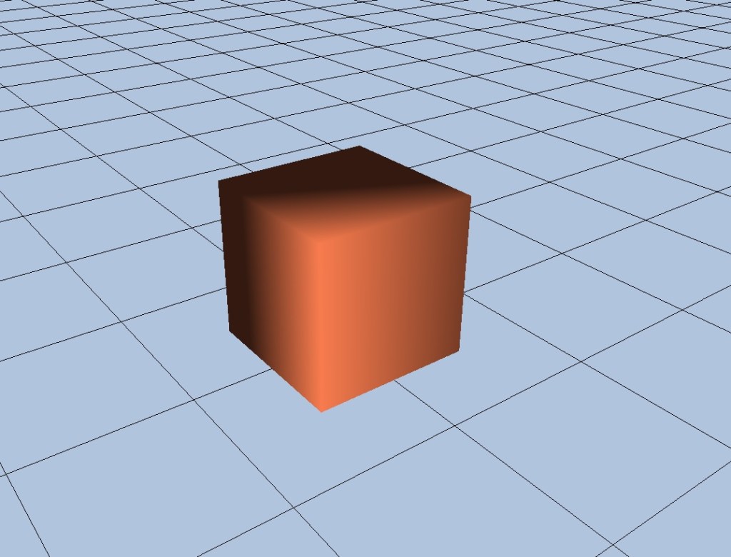
The image above (provided it’s displaying correctly) represents the end of Chapter 1. It shows a complete start-up of DirectX with everything needed to use its most fundamental features, and also contains proper rendered geometry using both a vertex and pixel shader, and all adapted over to containment within the project we have been building up to this point. That means it isn’t just running someone else’s code, it’s now working standalone in our own project, albeit with a lot of code carefully copied and pasted over from the recommend textbook (“3D Game Programming With DirectX 12” – By Frank Luna).

Porting it over was not a whole lot of fun, and I encountered many bugs and lessons about how much harder it is than you might think, to port existing code into your own project. It’s easy to underestimate just how much of it you’ll need, and lots of things suddenly stop working.

To get this far I’ve had to cover all of Chapter 5 and 6 in the recommended textbook. I also had to go back and cover Chapters 1 to 3. There is no way I’m going to attempt to describe all the elements of that here. Some of the math I still don’t understand, despite having a lengthy formal education. Much of it is not required to be understood precisely however, as DirectX contains built-in functions that do it for you, but you still need a reasonable grasp of what is happening. If you’re alright with vector and matrix math it shouldn’t be too bad (I was ok with those parts) but some of the concepts go quite a bit beyond that.

Chapter 5 deals mostly with the maths stuff and the rendering pipeline, building on knowledge from Chapters 1 to 3. You may recall from the previous chapter I stated we do not need to worry about the rendering pipeline. Well I kind of lied. We need to know quite a bit about it actually, but I didn’t want to start mentioning that sort of stuff in a chapter that was primarily focussed on just getting DirectX started. Anyone reading this blog rather tentatively would have probably bounced off straight away if I’d started discussing that stuff there.

Chapter 6 deals more with the protocol specific stuff needed to initialise everything you need, and how to prepare shader input and compile shaders.

I won’t be discussing anything too specific about either of those chapters here. I’ll leave that up to the textbook author.

What this blog chapter will contain is a few pointers about things I felt are worth highlighting from those textbook chapters, the means by which I’ve implemented the code in our own project, and some of the bugs I encountered along the way. I’ve also done some exploratory work getting models out of Blender, and how to cope with Blender’s different co-ordinate system to DirectX. That might be jumping the gun though. I may leave that to later chapters.

Chapter 5 in the textbook shows how to convert from one co-ordinate system to another co-ordinate system, and I wrote a program in Code::Blocks to test it out. It worked well, and I was pleased I was able to implement one of the concepts in the the textbook in my own little side project. We’ll need this if we ever start exporting models out of Blender.

For now though we’ll begin by discussing some of the concepts explained in the textbook that we need to grasp to understand how rendering 3D geometry is possible.

Assuming you’re up to speed on vectors and matrices (or have read the textbook Chapters 1 to 3 thoroughly) you’ll know that vectors can describe a displacement or a point, and that matrices can be used to transform vectors.

Note from the book how important the worldViewProjection matrix is. I had a hard time dealing with this until I was able to break it down into parts. Each part (world, view, projection) has its own matrix to describe the transformation it represents. What it’s ultimately transforming are the vertices that make up the geometry of any given object, namely a cube for example – like the one in the picture above. That cube has eight vertices. Each one gets assembled in the rendering pipeline and pumped through the vertex shader.

So the world part is just that. How much the original object has been scaled, rotated and translated into world space. Note from the book that matrix multiplication is associative. That means one transformation (say a scale for example) made as a 4 x 4 matrix multiplied by another transformation (a rotation for example) made as a 4 x 4 matrix will result in just one 4 x 4 matrix that contains both effects in just one matrix.

So the world matrix is one matrix that represents all 3 effects of scale, rotation and translation.

The next thing to consider is the camera. This is where things get a bit stranger than you would first expect. Whilst we are rendering stuff in three dimensions, our computer monitors are obviously just a two dimensional screen. So if you consider a 3D scene with an object (or several objects) placed in it at a certain place and rotation, imagine say just a cube sitting at the origin (0, 0, 0), we need to decide where our camera is going to be in that scene. What that camera “sees” will eventually be what’s shown on our monitor.

You can think of a camera as being a point in 3D space pointing at another point in 3D space. Imagine our camera is a CCTV camera monitoring an exit at a building somewhere. We can walk up to that scene in real life and see that the camera has a fixed position (up on the wall somewhere) and is pointing at another position (the exit door).

If you’ve ever played computer/video games you’ve looked through rendering API cameras many, many times. You probably just didn’t know how the view you see on the monitor was constructed behind the scenes. Well now you’re going to have to consider it. To put it in somewhat abstracted terms our “camera” is our “monitor’s” view into the 3D scene on our computer. It’s actually our responsibility to convert the geometry (vertices) in the scene into the camera’s co-ordinate system. So after all the world matrix stuff is done and the vertices are where they should be in our scene, we then have to find what their co-ordinates are relative to the camera, not the world.

For example if a vertex was placed a long way away from the origin in world space it would have large numbers for its co-ordinates, but if we placed our camera very close to it, it would have small numbers for its co-ordinates. In our security camera example this would be the co-ordinates of the four points of the exit door on the camera screen. If we looked through the security camera’s output on a remote monitor the z-axis would point straight out of it, the x-axis off to the right, and the y-axis straight up. And the co-ordinates wouldn’t be all that big in size as they’d all fit on the screen.

This change in co-ordinates from one system (world) to another (camera) is calculated by a matrix. This matrix is called the view transform. So we can now account for the second part of the worldViewProjection matrix. I won’t discuss how it’s done here, you can read the book for that. But that’s the essential concept of it.

Even if you can’t quite grasp that you’ll be saved anyway by the DirectX function XMMatrixLookAtLH(), as it does it for you. Quoting an example call from the book:

// sets a camera on the floor (note y component is zero and y points straight up)
// at 45 degrees between the x and z axis (both x and z components are 1)
// the last component is set to 1 as this is a position not a vector (see book for
// details)
XMVECTOR pos = XMVectorSet(1.0f, 0.0f, 1.0f, 1.0f);

// sets a vector to (0, 0, 0) which is the origin, so this camera will be pointed at
// the origin (0, 0, 0)
XMVECTOR target = XMVectorSetZero();

// see book for details about what this means (y axis is usually used as "up")
XMVECTOR up = XMVectorSet(0.0f, 1.0f, 0.0f, 0.0f);

// the final resultant matrix we want - to change world co-ordinates into
// camera co-ordinates
XMMATRIX view = XMMatrixLookAtLH(pos, target, up);

The last matrix to consider is the projection matrix. This is one of a few places I was rather lost when it came to the math. This is discussed in Chapter 5 of the book on page 182 onwards. I will revisit it again several times in the hope I can really pin it down, but for now I’ll make do with the DirectX function that computes it for us.

In essence though, a projection matrix recreates what you see with the human eye. Imagine looking down a long path lined by trees that were planted in identical spots either side of the path. Absolute mirror images of each other. In reality they are all in a straight line parallel to each other right to the end, but that’s not what you see with the human eye. You will see them begin to converge near the end of the path way off in the distance. They will appear closer together even though they are the exact same distance apart as the trees you are currently stood next to.

That’s what the projection matrix does. It performs the last remaining conversion that takes vertices in world space co-ordinates (world), transformed to camera space co-ordinates(view), and then arranges them so they fit the real world distance perspective model (projection).

Once already in camera co-ordinates (view space), the projection matrix probably doesn’t alter the vertex co-ordinates all that much. The effect is subtle, yet dramatic though. If it were missing it would probably bother your eye a great deal, without you immediately knowing why.

I mentioned View Frustums in the header some ways above. The frustum and projection matrix and very much interlinked. You can think of a frustum as a pyramid with the top knocked off. Where the top has been knocked off is the near plane, and the base of the pyramid is the far plane. The angle at which the lines of the pyramid leave its point origin (the top) and meet its base (in both vertical and horizontal directions), as well as the depth of the near plane (the point where we knock the top off) all define the view frustum. The book details these far better than I can so I’ll leave a proper explanation to the author. This short description just made however, roughly describes what it is and gives some insight into how the projection matrix is made.

The best way to see exactly how the code is implemented is of course, to study the source code, which is included in a download at the end. There are a few things I’d like to mention though. Note also I expect you to know what a Normal vector is during this explanation. If you’ve read the textbook chapters you’ll know what that is.

The textbook contains an exercise where you are requested to put some of the vertex data in different buffers. The source code for this chapter is done with the methods needed to complete that exercise.

That’s a long winded way of saying the vertex data pumped into the vertex shader comes from two different vertex buffers, when you could easily do it by only using one (but we wouldn’t be learning anything interesting). Assuming you’re familiar with Chapter 6 in the textbook have a look at the code below:

void D3DRenderer::BuildShadersAndInputLayout()
{
    HRESULT hr = S_OK;

    mvsByteCode = d3dUtil::CompileShader(L"Shaders\\color.hlsl",
                                         nullptr, "VS", "vs_5_0");
    mpsByteCode = d3dUtil::CompileShader(L"Shaders\\color.hlsl",
                                         nullptr, "PS", "ps_5_0");

    mInputLayout =
    {
        { "POSITION", 0, DXGI_FORMAT_R32G32B32_FLOAT, 0, 0,
         D3D12_INPUT_CLASSIFICATION_PER_VERTEX_DATA, 0 },

	{ "NORMAL", 0, DXGI_FORMAT_R32G32B32_FLOAT, 0, 12,
         D3D12_INPUT_CLASSIFICATION_PER_VERTEX_DATA, 0},

        { "COLOR", 0, DXGI_FORMAT_R32G32B32A32_FLOAT, 1, 0,
         D3D12_INPUT_CLASSIFICATION_PER_VERTEX_DATA, 0 }
   }

}

Note that the POSITION and NORMAL semantics are both tied to slot 0, and the COLOUR semantic is tied to slot 1. The slot number is the fourth parameter in the creation of each D3D12_INPUT_ELEMENT_DESC element, where mInputLayout is an array (vector) of D3D12_INPUT_ELEMENT_DESC’s.

That means the position and normal data will be pumped through slot 0, and the color data pumped through slot 1. Also note the byte offsets in the fifth parameter for each element are different. For position and normal it goes 0, then 12. For color it’s just 0. That means in the first slot (slot 0) the position is read at byte offset 0, and then the normal is read at byte offset 12. In the second slot (slot 1) only color is read starting at byte offset 0.

If you then study the .cpp file “Vertices & Geometry.cpp” you’ll see that the position and normal data get put into their own vertex buffer, and the color data gets put into its own vertex buffer too. For convenience we’re not discussing the index buffer here, only the vertex buffers.

std::array<Vertex, 8> vertices = 
{ 
    Vertex({ XMFLOAT3(-1.0f, 0.0f, -1.0f), XMFLOAT3(-0.57735f, -0.57735f, -0.57735f) }),
    .... create remaining vertices
}

std::array<std::uint16_t, 36> indices =
{
    // front face
    0, 1, 2,
    .... create remaining indices
}
std::array <Color, 8> colors;
for (uint16_t i = 0; i < 8; i++)
{
	colors[i].Color = XMFLOAT4(Colors::Coral);
}   .... create colors


const UINT vbByteSize = (UINT)vertices.size() * sizeof(Vertex);
const UINT ibByteSize = (UINT)indices.size() * sizeof(std::uint16_t);
const UINT cbByteSize = (UINT)colors.size() * sizeof(Color);

mBoxGeo = std::make_unique<MeshGeometry>();

mBoxGeo->Name = "boxGeo";

ThrowIfFailed(D3DCreateBlob(vbByteSize, &mBoxGeo->VertexBufferCPU));
CopyMemory(mBoxGeo->VertexBufferCPU->GetBufferPointer(), vertices.data(), vbByteSize);

ThrowIfFailed(D3DCreateBlob(ibByteSize, &mBoxGeo->IndexBufferCPU));
CopyMemory(mBoxGeo->IndexBufferCPU->GetBufferPointer(), indices.data(), ibByteSize);

ThrowIfFailed(D3DCreateBlob(cbByteSize, &mBoxGeo->ColorBufferCPU));
CopyMemory(mBoxGeo->ColorBufferCPU->GetBufferPointer(), colors.data(), cbByteSize);

mBoxGeo->VertexBufferGPU = d3dUtil::CreateDefaultBuffer(md3dDevice.Get(),
	mCommandList.Get(), vertices.data(), vbByteSize, mBoxGeo->VertexBufferUploader);

mBoxGeo->IndexBufferGPU = d3dUtil::CreateDefaultBuffer(md3dDevice.Get(),
	mCommandList.Get(), indices.data(), ibByteSize, mBoxGeo->IndexBufferUploader);

mBoxGeo->ColorBufferGPU = d3dUtil::CreateDefaultBuffer(md3dDevice.Get(),
	mCommandList.Get(), colors.data(), cbByteSize, mBoxGeo->ColorBufferUploader);

mBoxGeo->VertexByteStride = sizeof(Vertex);
mBoxGeo->VertexBufferByteSize = vbByteSize;

mBoxGeo->IndexFormat = DXGI_FORMAT_R16_UINT;
mBoxGeo->IndexBufferByteSize = ibByteSize;

mBoxGeo->ColorByteStride = sizeof(Color);
mBoxGeo->ColorBufferByteSize = cbByteSize;

I also modified the MeshGeometry struct you can find in the very useful “d3dUtil.h” file written by the textbook author, to include an extra vertex buffer for the color data. Otherwise the code above would fail.

struct MeshGeometry
{
    std::string Name;

    Microsoft::WRL::ComPtr<ID3DBlob> VertexBufferCPU = nullptr;
    Microsoft::WRL::ComPtr<ID3DBlob> ColorBufferCPU = nullptr;
    Microsoft::WRL::ComPtr<ID3DBlob> IndexBufferCPU  = nullptr;

    Microsoft::WRL::ComPtr<ID3D12Resource> VertexBufferGPU = nullptr;
    Microsoft::WRL::ComPtr<ID3D12Resource> ColorBufferGPU = nullptr;
    Microsoft::WRL::ComPtr<ID3D12Resource> IndexBufferGPU = nullptr;

    Microsoft::WRL::ComPtr<ID3D12Resource> VertexBufferUploader = nullptr;
    Microsoft::WRL::ComPtr<ID3D12Resource> ColorBufferUploader = nullptr;
    Microsoft::WRL::ComPtr<ID3D12Resource> IndexBufferUploader = nullptr;

    ....struct continues
}

I won’t explain what the Uploader buffers or d3dUtil::CreateDefaultBuffer() functions are doing here. At this point it is expected you have read the book and are up to speed on this.

So, after a lot of code, and a lot of memory copying, we have a load of data in two different buffers that live on the GPU. One contains vertex position and normal data, and the other color data. So how then do we assemble all this correctly so the input to the vertex shader can correctly associate the right data to the semantics defined in the mInputLayout array shown above (re-produced below for convenience):

mInputLayout =
    {
        { "POSITION", 0, DXGI_FORMAT_R32G32B32_FLOAT, 0, 0,
         D3D12_INPUT_CLASSIFICATION_PER_VERTEX_DATA, 0 },

	{ "NORMAL", 0, DXGI_FORMAT_R32G32B32_FLOAT, 0, 12,
         D3D12_INPUT_CLASSIFICATION_PER_VERTEX_DATA, 0},

        { "COLOR", 0, DXGI_FORMAT_R32G32B32A32_FLOAT, 1, 0,
         D3D12_INPUT_CLASSIFICATION_PER_VERTEX_DATA, 0 }
   }

In the big function that draws everything (imaginatively named “Draw”) we use a function that binds the resource (one of the two vertex buffers containing data) to the rendering pipeline. In particular we can bind a resource to a specific vertex input slot. You may remember some time ago in this blog we discussed descriptors (also termed “views”) and how they are needed to bind resources to the rendering pipeline. This is another example of this. In the Draw() function there are two lines that arrange all of this:

mCommandList->IASetVertexBuffers(0, 1, &mBoxGeo->VertexBufferView());
mCommandList->IASetVertexBuffers(1, 1, &mBoxGeo->ColorBufferView());

The function IASetVertexBuffers() takes 3 arguments. The second is how many descriptors/views we are going to use to bind resources to the pipeline, and the third is a pointer to an array of the views themselves. We are only binding one resource to the pipeline per IASetVertexBuffers() function call so the second parameter is always 1. The third parameter is an actual view constructed “on the fly” so to speak. It comes from the MeshGeometry struct which returns a view to the GPU buffer it has stored, which it can acquire a pointer to. Here’s a small snippet (see the source code for a more complete understanding):

D3D12_VERTEX_BUFFER_VIEW VertexBufferView()const
{
	D3D12_VERTEX_BUFFER_VIEW vbv;
	vbv.BufferLocation = VertexBufferGPU->GetGPUVirtualAddress();
	vbv.StrideInBytes = VertexByteStride;
	vbv.SizeInBytes = VertexBufferByteSize;

	return vbv;
}	

That’s why the MeshGeometry struct mentioned some ways above (in the big code section where we initialised all the buffers & geometry) needed all that data about the buffers it had stored. Namely their ByteStride and BufferByteSize. All this view does, is just hold an address for the buffer on the GPU, a record of its total size, and a record of how big each vertex element in the buffer is, so the computer knows how much data to read at a time (the ByteStride).

Note that unlike other views/descriptors vertex and index buffers views do not live in heaps.

Returning to the IASetVertexBuffers() function, when this has been called twice, once for the vertex buffer (containing position and normal data), and once for the color buffer (which is strictly speaking also a vertex buffer we just called it something different), all the “stuff” in VertexBuffer is bound to slot 0, and all the “stuff” in ColorBuffer is bound to slot 1.

That’s what the first parameter to the IASetVertexBuffers() does. It determines which input slot to set a view to. It uses the view to bind the data the view refers to, to an input slot.

So now when the computer consults mInputLayout, it goes to slot 0, starts at byte 0 and expects to find 12 bytes of data (a 3 element vector of floats representing position data – DXGI_FORMAT_R32G32B32_FLOAT).

Then it stays on slot 0 and at the 13th byte (which has number 12 for a zero indexed system), continues to read another 12 bytes of data (a 3 element vector of floats representing a normal vector – DXGI_FORMAT_R32G32B32_FLOAT).

Then lastly it changes slots to slot 1 and starting at byte 0, reads 12 bytes containing color data (another DXGI_FORMAT_R32G32B32A32_FLOAT).

Have a look again at the mInputLayout array, and bear in mind byte indexes will begin at zero, not one.

mInputLayout =
{
	{ "POSITION", 0, DXGI_FORMAT_R32G32B32_FLOAT, 0, 0, D3D12_INPUT_CLASSIFICATION_PER_VERTEX_DATA, 0 },
	{ "NORMAL", 0, DXGI_FORMAT_R32G32B32_FLOAT, 0, 12, D3D12_INPUT_CLASSIFICATION_PER_VERTEX_DATA, 0},
	{ "COLOR", 0, DXGI_FORMAT_R32G32B32A32_FLOAT, 1, 0, D3D12_INPUT_CLASSIFICATION_PER_VERTEX_DATA, 0 }
};

Because we’ve loaded the two different buffers with the right data (one for position and normal, the other for color), and bound them to the correct slots using the IASetVertexBuffers() function, the computer now simply finds all the data we loaded into the two buffers at the correct spot, and can now relate the data it finds to the correct semantic, either POSITION, NORMAL, or COLOR.

So when the shader runs later (HLSL snippet from our shader below):

struct VertexIn
{
    float4 Color : COLOR;
    float3 PosL  : POSITION;   
    float3 Norm  : NORMAL;
};

these semantics all point to the right data, and we can use them in our shader program.

At least I hope that’s the case anyway. After having gone out on a limb like that I’d look awfully silly if that description turned out to be wrong for some bizarre reason I’d overlooked in my tests. Extensive testing and checking on my end strongly suggests I needn’t worry though 🙂

So from this we can see that’s how we assemble data in different buffers in a way that lands where it should be in the vertex shader.

And that’s probably enough for a description of anything relevant in how I implemented the code. For anything else you can simply study (or stare at) the source code. Other than what’s described above, it follows the original author’s code very closely and just makes adaptations to our project wherever it has to. There are quite a lot of adaptations however, but they are too numerous and too trivial to discuss here. Study the source code for a better understanding of what they are.

Vertex normals are another mess we have to sort out. This project in its current state uses vertex normals, rather than face normals. Take our cube for example. It has 8 vertices and 12 faces. We use an index list to draw 12 faces from 8 points. I’ll assume you’ve read the relevant textbook chapters and know what an index list is.

If we really wanted to (and in some ways it would be easier) we could make our cube of 12 faces (like we already have) but made from 36 vertices. 3 per face. This would obviously cause duplicate vertices to exist at similar points, but it would make lighting the cube very easy. All triangles (faces) would just have one normal perpendicular to the plane the 3 vertices lay in.

You would still need an index list to draw this cube, but lighting it would be easy as each face would have its own normal. If we moved a light around this cube it would light very naturally and nicely indeed.

So why not do that? Well…. it takes a lot more vertices than you really need to do it which wastes memory and is probably slower, and… I have bad memories appearing of when I last gave up on all this rendering stuff over 12 years ago in early 2012. I used the duplicate vertices method. I even exported models out of Blender using them, although I can’t remember how. When I came to animate things though I realised I was in trouble.

Animating things may have changed since, and to be honest I haven’t kept up, but what I remember is when you tried to animate meshes with duplicate vertices they always had tears in them. That’s because an animated “group” (say a character’s arm) is just a collection of vertices. You then transform only those vertices and not the rest of the model to make the animation. If you’re using duplicate vertices then the vertices in the animated group aren’t “anchored” to anything and tears appear. I may have missed something I don’t know, but I always knew if I ever returned to this I would be using minimal vertices to describe a model (no duplicates), and vertex normals not face normals.

Vertex normals can be used with a minimal amount of vertices, such as for our cube only having 8 vertices yet 12 faces. It will (I hope) work better with animations later and also cut down on computations and memory use.

Are there any downsides? Yes there are. Vertex normals have to be computed as an average of all the face normals associated with them. Picture a vertex on our cube. It’s right on the point part where several triangles meet. We need just one normal to represent the vertex as we’re only allowed one normal per vertex. But how do you do that given that there are potentially several triangles in an index list using that vertex that are all perpendicular to each other?

That’s where you have to use an average. In a later chapter I’ll show a vertex normal averaging algorithm. I’ve already run it and it’s pretty good although it suffers a bit when used on a cube. There are revisions I can make to it though which may solve this. Without going into much detail I’ll show a picture here from Blender where I’ve drawn what the averaged vertex normals look like on a cube with 8 vertices and 12 faces:

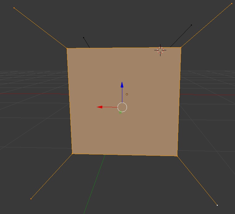
Notice how they’re pretty much at 45 degrees to every axis. This is what we would expect from a cube, given that every side is perpendicular to the next. The normals you see here are the same normals used to light the cube in this project. It’s why despite the light vector that orbits the cube being flat (y component is zero) and facing directly at the cube face, you can still see some light on the upper and lower surfaces. See the picture at the start of this chapter for an idea.

If these normals were dead flat you wouldn’t see any light at all on the upper and lower surfaces. You also wouldn’t see any light on 2 sides of the cube either!

Cutting a long story short we’re going with vertex normals for this project. They have limitations, but they’re a better choice in the long run, and give a good averaged result. I’ll detail vertex normal computation algorithms in a later chapter.

The last thing to discuss for this part is the shader. No discussion at all will be made about shader compilation or root signatures. For that consult the textbook and the source code. Assuming you know what the dot product of two vectors is, and building on knowledge from the book and this blog chapter, understanding this HLSL shader code should be straight forward:

//***************************************************************************************
// color.hlsl by Frank Luna (C) 2015 All Rights Reserved.
//
// Transforms and colors geometry.
//***************************************************************************************
// Made some small additions to include directional light - Chris H 5/10/24

cbuffer cbPerObject : register(b0)
{   
    float3 light;    
    float4x4 gWorldViewProj; 
};

struct VertexIn
{
    float4 Color : COLOR;
    float3 PosL  : POSITION;   
    float3 Norm  : NORMAL;
};

struct VertexOut
{
    float4 PosH  : SV_POSITION;
    float4 Color : COLOR;
    float3 Norm  : NORMAL;
};

VertexOut VS(VertexIn vin)
{
    VertexOut vout;

    // Transform to homogeneous clip space.
    vout.PosH = mul(float4(vin.PosL, 1.0f), gWorldViewProj);

    vout.Color = vin.Color;
    vout.Norm  = vin.Norm;    
    return vout;
}

float4 PS(VertexOut pin) : SV_Target
{   
    // Use Below For Per Pixel Directional Light
    float temp = max(dot(light, pin.Norm), 0);
    return (pin.Color * (temp + 0.2) );
}

The vertex shader takes the input vertex position and transforms it using the gWorldViewProj matrix fed in from the constant buffer (see textbook for details about what a constant buffer is). The vertex is now in camera co-ordinates and adjusted for perspective. The pixel shader then performs the dot product of the vertex normal with the light direction vector and assigns the value to variable temp. Finally we return the pixel color multiplied by the dot product result with a 0.2 addition to add some ambient light to all pixels and perhaps a touch of glare on the cube edge pixels (where the scalar from the dot product is already high).

Note the lighting is done in the pixel shader not the vertex shader. This is computationally more expensive but gives a very nice gentle light motion around the cube as the light is computed per pixel. Most likely as this project progresses we will drop this in favour of it being done in the vertex shader for performance reasons. It won’t look quite as nice though.

I’ll keep this part concise as I’ve written an awful lot already. I certainly did encounter bugs whilst writing some of this code and also when moving parts from the original author’s code into our project.

One of them was appalling. I made a new function in the render interface that allowed me to access the Update() function in the render dll, as part of the D3DRenderer class. All it did was forward on an instruction to call the D3DRenderer member function Update(). There are two Update() functions in the D3DRenderer class, one is an over ride from the abstract interface class, the other is a typical member function:

class IMPORT_EXPORT D3DInterface
{
public:
    
    virtual void    Update() = 0;

    ....class continues
}

class D3DRenderer : public D3DInterface
{
public:
    void    Update()override;

private:
    // Drawing and bound view retrieval functions
    void    Update(const GameTimer& gt);

    ....class continues
}

....later on

void D3DRenderer::Update()
{      
    // mTimer is of type GameTimer and is a member of class D3DRenderer 
    Update(mTimer);
    return;
}

void D3DRenderer::Update(const GameTimer& gt)
{
    ....function body
}

When I tried to call this function in the main application (the one that loads this dll file) it crashed horribly. In fact I could only call a few functions in the render interface despite there being several declared. It was like it did not recognise the interface to the dll or even the dll at all at runtime. Or worse only parts of it….

When I ran the debugger tool and it came across the runtime error it sent me to a file that belonged in part 3 in my hard drive. The problem being this was part 4. And I had compiled the dll file from the project in the part 4 folder also.

I’m still bemused as to exactly how this took place, but I know it had something to do with the fact I just copied and pasted the old part 3 (code for previous blog chapter) into a new folder named part 4 and then just altered headers and source files to suit.

Because the computer was referencing an older version of the dll it could not find any of the new functions I’d added to the interface which it attempted to call in the dll.

The lesson being, don’t just copy and paste a project, unless you really know your way around the IDE. I fixed this by making a brand new project and adding the necessary files and then compiling from there. It was a frighteningly confusing error, and one I would not want to repeat!

The only other noteworthy bug came after I got everything to work and the screen was rendering stuff. It was horribly slow. Really chunky. I was beginning to wonder if it was not really possible anymore to use a dll file to contain a render library, or if I’d screwed something up in the window message loop. My thoughts ran wild.

As it turned out all I needed to do was call the Reset() method belonging to the GameTimer object. The GameTimer object is needed to compute the light source direction so you see the light nicely move around the cube. I suspect if you don’t reset it, it’s using numbers way too large for calculations resulting in lower performance or accuracy loss. Anyways, once rooted out this was an easy fix.

Well, that’s that for now, I hope that was useful to you. There’ll be more interesting stuff to follow in later chapters, but I don’t know when they will be available. I have some work to do yet on learning some optimisation tricks the textbook author has made, which I don’t yet fully understand. Anyways, download the latest project revision if you wish from the following link:

Article 4 (Complete).zip

Thank you for reading 🙂

Chris H